plot_track() visualizes trajectory and footprint data from codetrack R objects in various ways, allowing for the plotting of trajectories, footprints, or both combined, with customizable aesthetics.
Usage
plot_track(
  data,
  plot = "FootprintsTrajectories",
  colours = NULL,
  cex.f = NULL,
  shape.f = NULL,
  alpha.f = NULL,
  cex.t = NULL,
  alpha.t = NULL,
  plot.labels = NULL,
  labels = NULL,
  box.p = NULL,
  cex.l = NULL,
  alpha.l = NULL,
  arrow.t = FALSE,
  arrow.size = 0.15,
  seq.foot = FALSE
)
Arguments
- data
A
trackwayR object. Seetps_to_track.- plot
Type of plot to generate. Options are
"FootprintsTrajectories"(default),"Trajectories", or"Footprints". Determines what elements are included in the plot.- colours
A vector of colors to be used for different trajectories If
NULL, defaults to black. The length of this vector should match the number of trackways in the data.- cex.f
The size of the points representing footprints. Default is
2.5. Ifseq.foot = TRUE, this controls the text size of footprint sequence numbers.- shape.f
A vector of shapes to be used for representing footprints in different trackways. If
NULL, defaults to19(solid circle). The length of this vector should match the number of trackways in the data.- alpha.f
The transparency of the points representing footprints. Default is
0.5.- cex.t
The thickness of the trajectory lines. Default is
0.5.- alpha.t
The transparency of the trajectory lines. Default is
1.- plot.labels
Logical indicating whether to add labels to each trackway. Default is
FALSE.- labels
A vector of labels for each trackway. If
NULL, labels are automatically generated from trackway names.- box.p
Padding around label boxes, used only if
plot.labelsisTRUE. Adjusts the spacing around the label text.- cex.l
The size of the labels. Default is
3.88.- alpha.l
The transparency of the labels. Default is
0.5.- arrow.t
Logical indicating whether to add an arrowhead at the end of each trajectory to verify direction. Default is
FALSE.- arrow.size
Numeric controlling the arrowhead size (in inches, passed to
grid::unit()). Default is0.15.- seq.foot
Logical indicating whether to display the footprint sequence numbers instead of footprint points. Default is
FALSE. This is useful to verify that footprints are in the correct order along each trackway. WhenTRUE, the size of the numbers is controlled bycex.f.
Value
A ggplot object that displays the specified plot type, including trajectories, footprints, or both, from trackway R objects. The ggplot2 package is used for plotting.
Details
The plot_track() function is designed as a diagnostic and exploratory tool.
Its primary purpose is to display the raw spatial data (footprint coordinates and
interpolated trajectories) that have been digitized, so that users can
visually confirm data integrity before conducting quantitative analyses. This
includes checking whether footprints are in the correct order, whether trackways are
oriented consistently, and whether interpolated trajectories align with the raw
footprint data.
Importantly, these plots are not intended to replace traditional ichnological illustrations. Hand-drawn maps and outlines often convey information that is not captured in raw coordinate plots, such as tridactyl morphology, manus/pes distinction, taxonomic attribution, or trackway orientation, and they frequently provide clearer and more communicative visual summaries of ichnological material.
By contrast, plot_track() focuses on plotting digitized data as they are,
without additional interpretation, stylization, or symbolic annotation. The goal is
to offer a reproducible, data-driven representation that complements, rather than
supplants, traditional methods. Users are encouraged to treat these plots as
quality-control visualizations that help detect potential errors or inconsistencies
in the raw data prior to downstream analyses, while continuing to rely on classical
ichnological illustrations for detailed morphological and taxonomic interpretation.
Author
Humberto G. Ferrón
humberto.ferron@uv.es
Macroevolution and Functional Morphology Research Group (www.macrofun.es)
Cavanilles Institute of Biodiversity and Evolutionary Biology
Calle Catedrático José Beltrán Martínez, nº 2
46980 Paterna - Valencia - Spain
Phone: +34 (9635) 44477
Examples
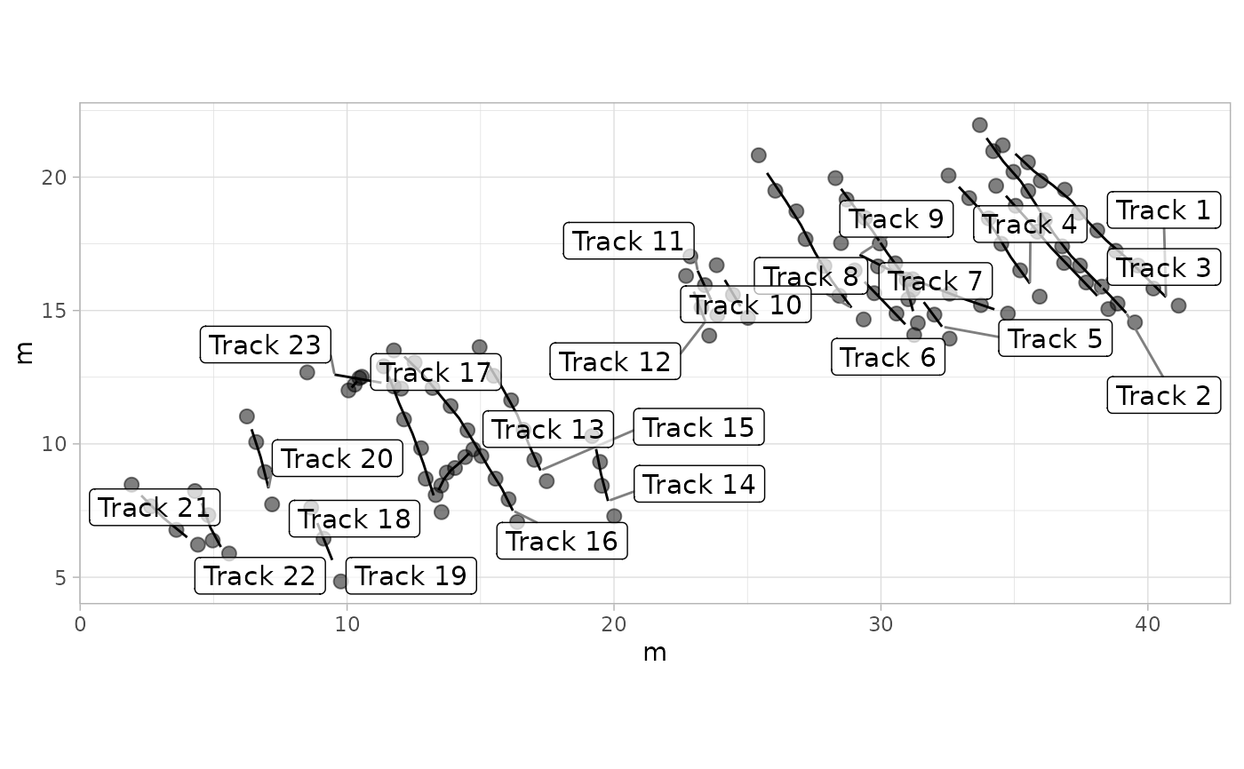
# Example 1: Basic Plot with Default Settings - MountTom Dataset
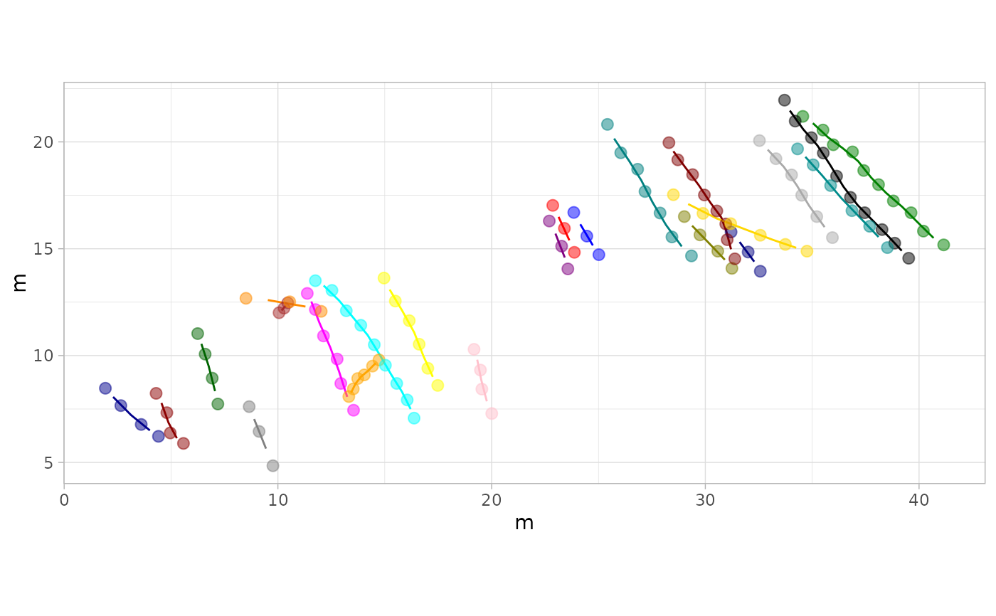
plot_track(MountTom)
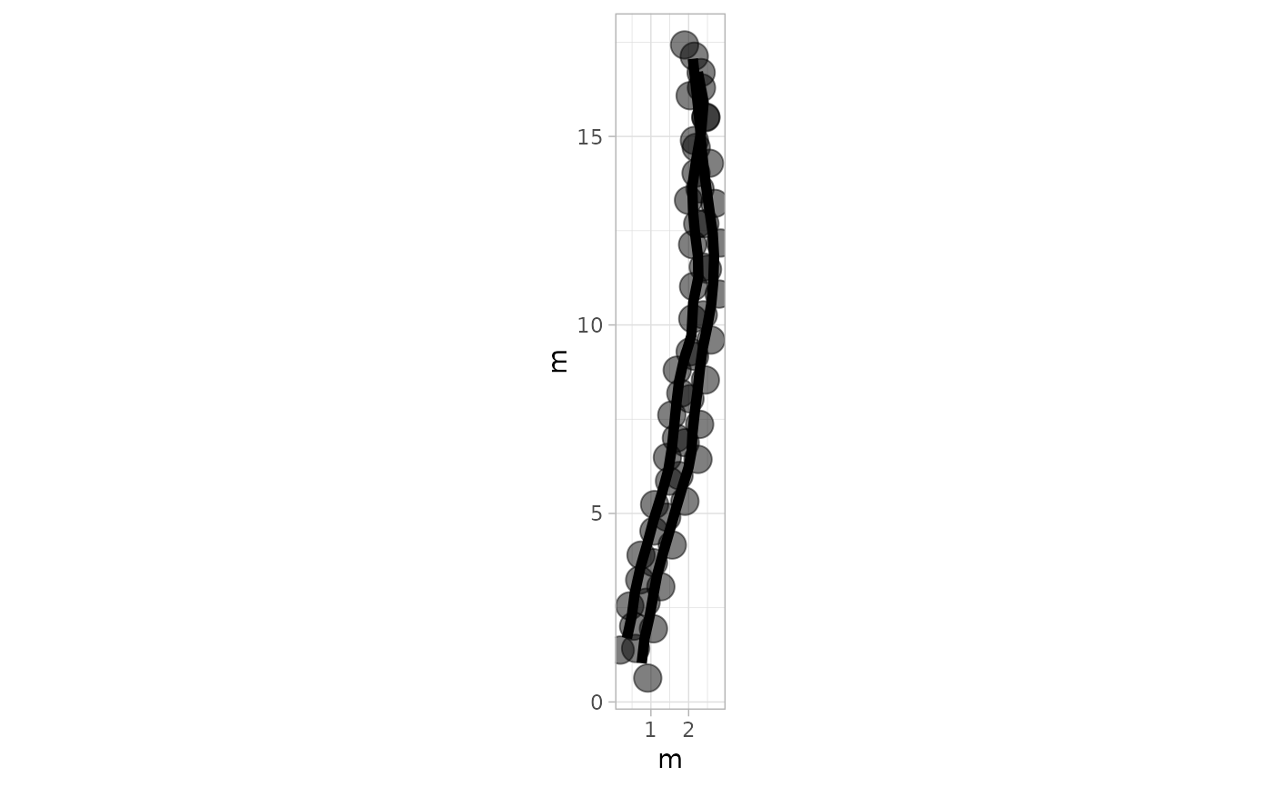
 # Example 2: Basic Plot with Default Settings - PaluxyRiver Dataset
plot_track(PaluxyRiver)
# Example 2: Basic Plot with Default Settings - PaluxyRiver Dataset
plot_track(PaluxyRiver)
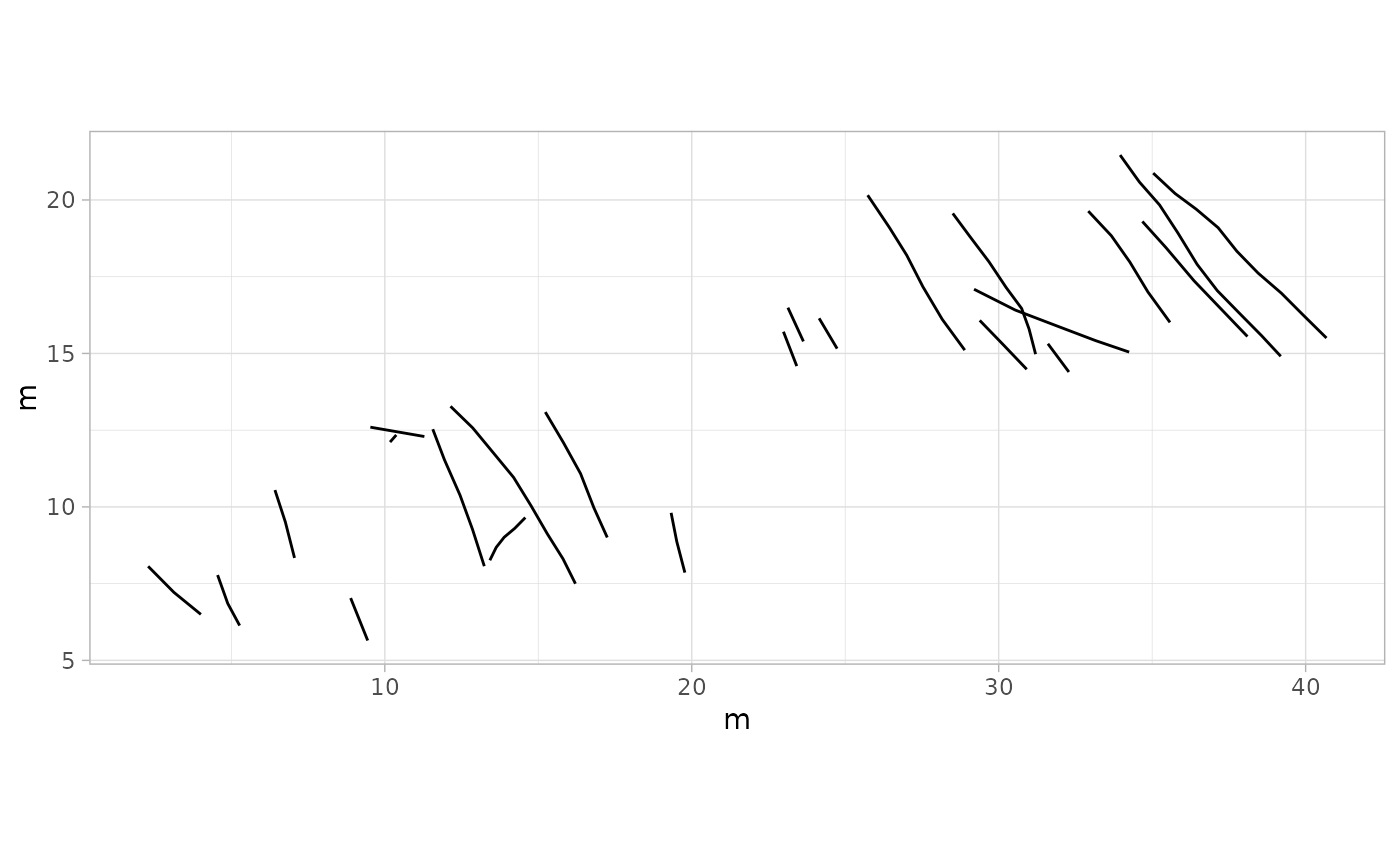
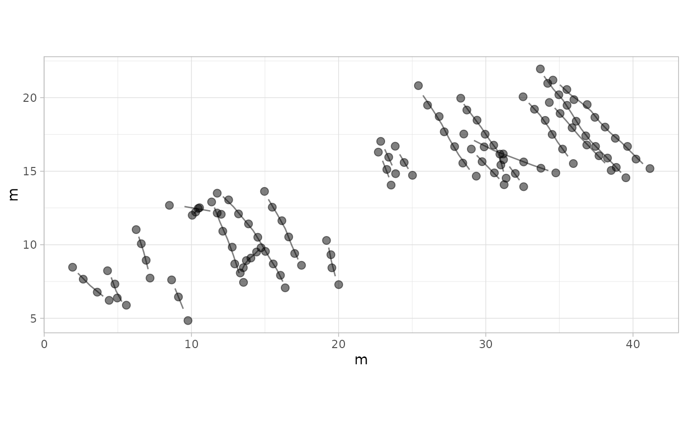
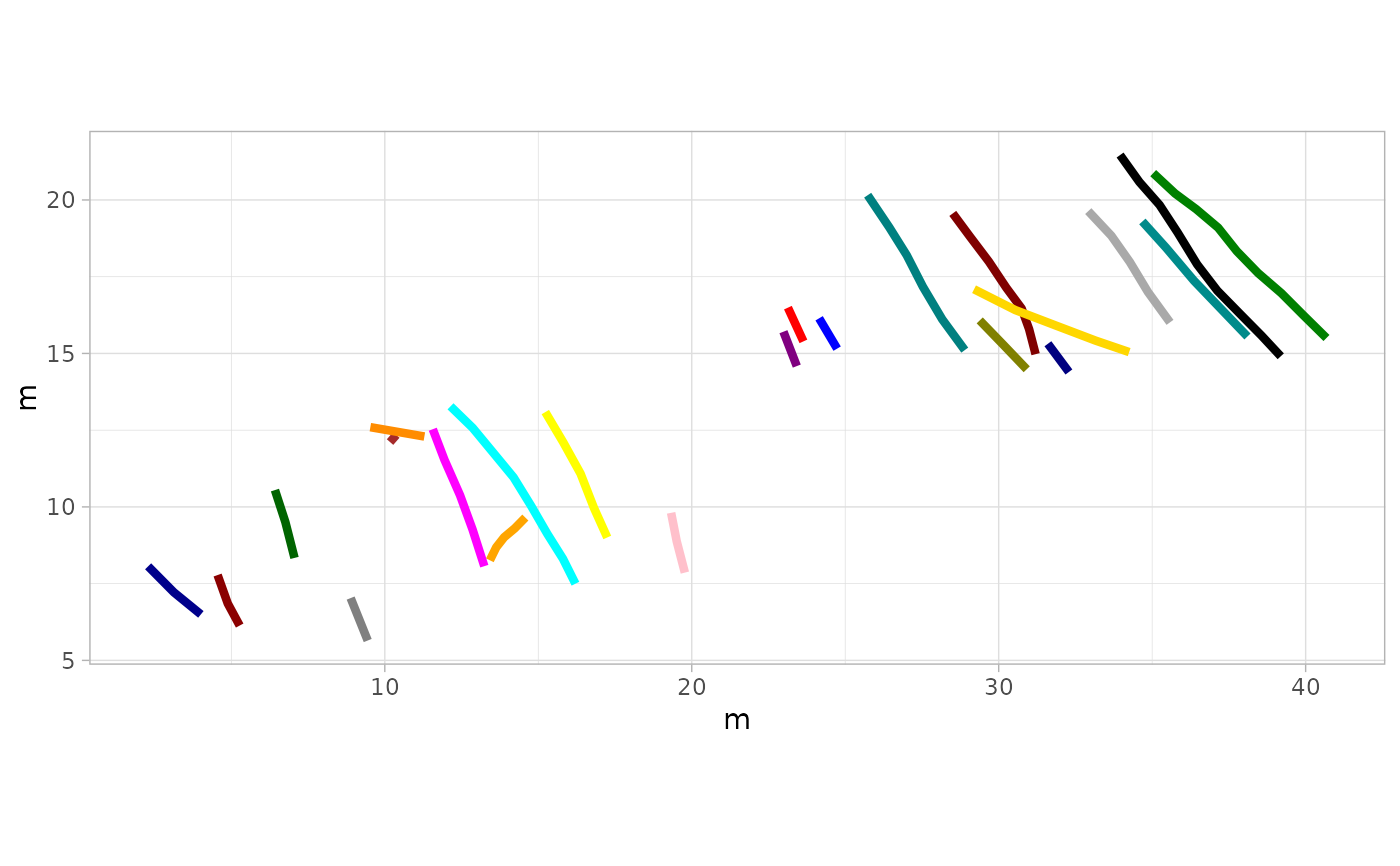
 # Example 3: Plot Trajectories Only - MountTom Dataset
plot_track(MountTom, plot = "Trajectories")
# Example 3: Plot Trajectories Only - MountTom Dataset
plot_track(MountTom, plot = "Trajectories")
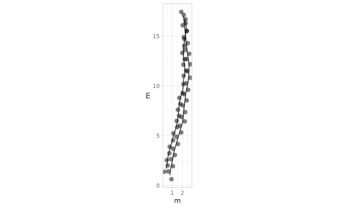
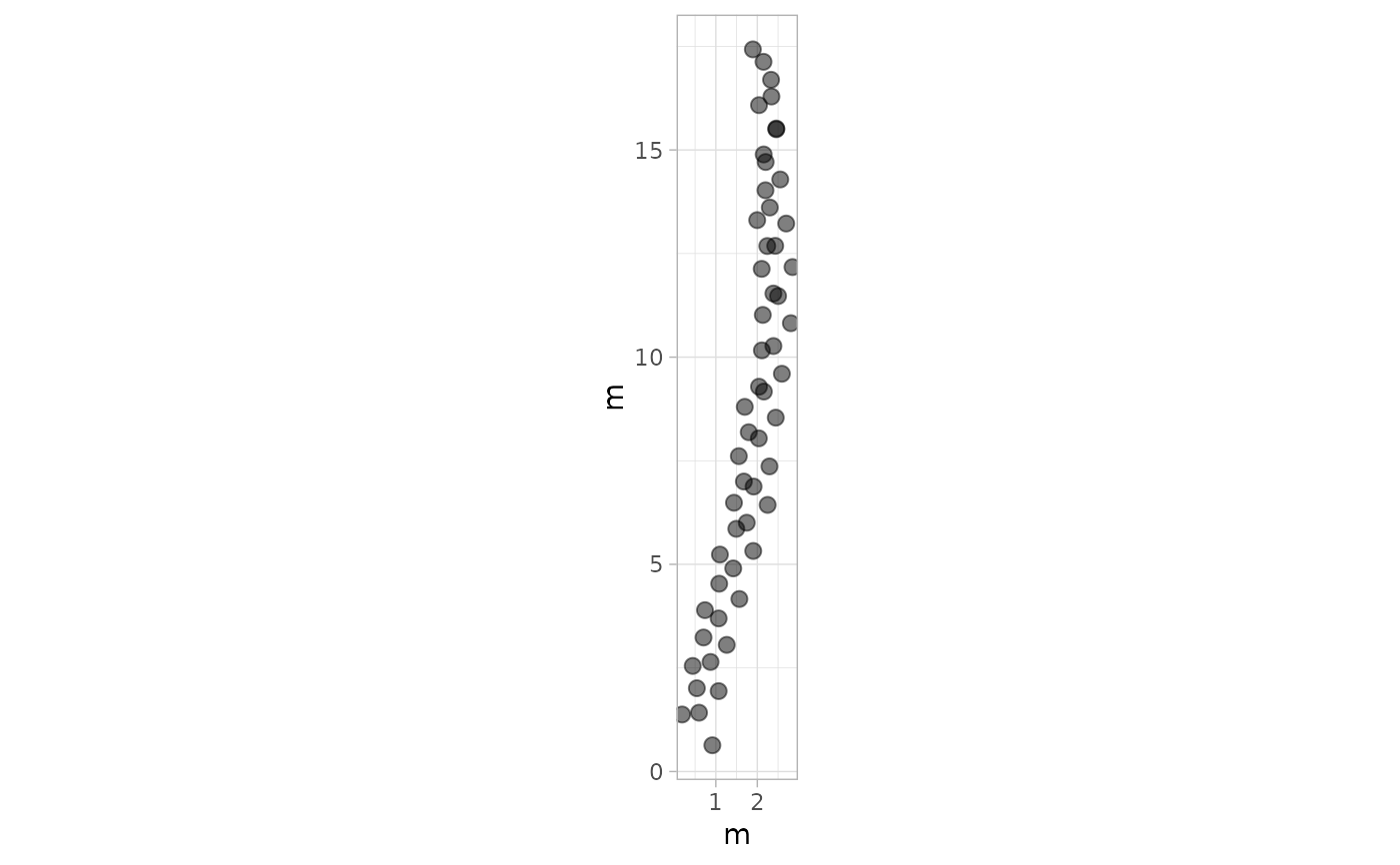
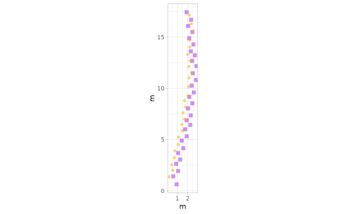
 # Example 4: Plot Footprints Only - PaluxyRiver Dataset
plot_track(PaluxyRiver, plot = "Footprints")
# Example 4: Plot Footprints Only - PaluxyRiver Dataset
plot_track(PaluxyRiver, plot = "Footprints")
 # Example 5: Custom Colors for Trajectories - MountTom Dataset
custom_colors <- c(
"#008000", "#0000FF", "#FF0000", "#800080", "#FFA500", "#FFC0CB", "#FFFF00",
"#00FFFF", "#A52A2A", "#FF00FF", "#808080", "#000000", "#006400", "#00008B",
"#8B0000", "#FF8C00", "#008B8B", "#A9A9A9", "#000080", "#808000", "#800000",
"#008080", "#FFD700"
)
plot_track(MountTom, colours = custom_colors)
# Example 5: Custom Colors for Trajectories - MountTom Dataset
custom_colors <- c(
"#008000", "#0000FF", "#FF0000", "#800080", "#FFA500", "#FFC0CB", "#FFFF00",
"#00FFFF", "#A52A2A", "#FF00FF", "#808080", "#000000", "#006400", "#00008B",
"#8B0000", "#FF8C00", "#008B8B", "#A9A9A9", "#000080", "#808000", "#800000",
"#008080", "#FFD700"
)
plot_track(MountTom, colours = custom_colors)
 # Example 6: Larger Footprints and wider Trajectories Lines - PaluxyRiver Dataset
plot_track(PaluxyRiver, cex.f = 5, cex.t = 2)
# Example 6: Larger Footprints and wider Trajectories Lines - PaluxyRiver Dataset
plot_track(PaluxyRiver, cex.f = 5, cex.t = 2)
 # Example 7: Semi-Transparent Footprints and Trajectories - MountTom Dataset
plot_track(MountTom, alpha.f = 0.5, alpha.t = 0.5)
# Example 7: Semi-Transparent Footprints and Trajectories - MountTom Dataset
plot_track(MountTom, alpha.f = 0.5, alpha.t = 0.5)
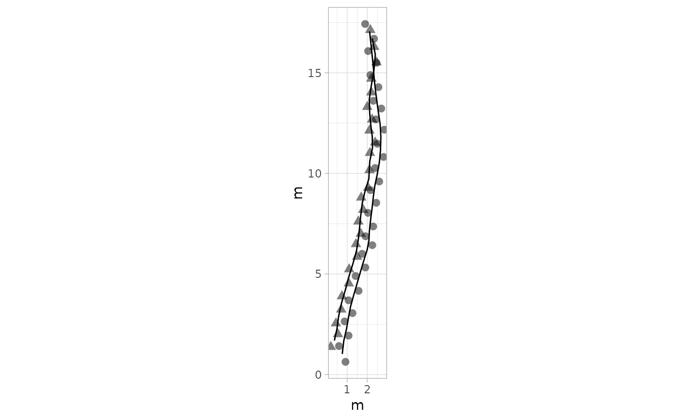
 # Example 8: Different Shapes for Footprints - PaluxyRiver Dataset
plot_track(PaluxyRiver, shape.f = c(16, 17))
# Example 8: Different Shapes for Footprints - PaluxyRiver Dataset
plot_track(PaluxyRiver, shape.f = c(16, 17))
 # Example 9: Plot with Labels for Trajectories - MountTom Dataset
labels <- paste("Trackway", seq_along(MountTom[[1]]))
plot_track(MountTom, plot.labels = TRUE, labels = labels, cex.l = 4, box.p = 0.3, alpha.l = 0.7)
# Example 9: Plot with Labels for Trajectories - MountTom Dataset
labels <- paste("Trackway", seq_along(MountTom[[1]]))
plot_track(MountTom, plot.labels = TRUE, labels = labels, cex.l = 4, box.p = 0.3, alpha.l = 0.7)
 # Example 10: Custom Colors and Shapes for Footprints Only - PaluxyRiver Dataset
plot_track(PaluxyRiver, plot = "Footprints", colours = c("purple", "orange"), shape.f = c(15, 18))
# Example 10: Custom Colors and Shapes for Footprints Only - PaluxyRiver Dataset
plot_track(PaluxyRiver, plot = "Footprints", colours = c("purple", "orange"), shape.f = c(15, 18))
 # Example 11: Wider Line Size & Custom Colors for Trajectories Only - MountTom Dataset
plot_track(MountTom, plot = "Trajectories", cex.t = 1.5, colours = custom_colors)
# Example 11: Wider Line Size & Custom Colors for Trajectories Only - MountTom Dataset
plot_track(MountTom, plot = "Trajectories", cex.t = 1.5, colours = custom_colors)
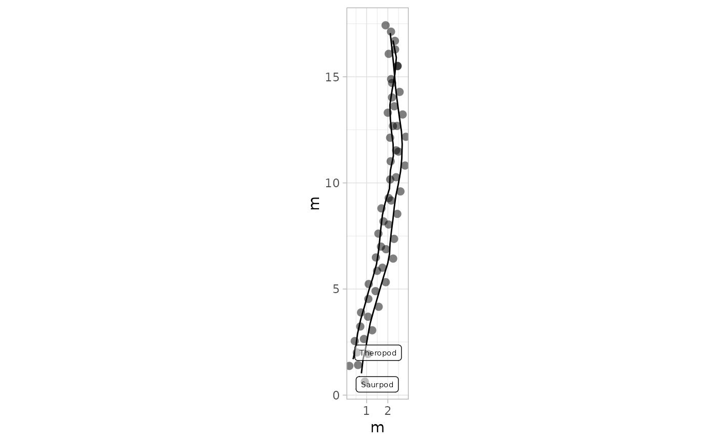
 # Example 12: Black Footprints and Trajectories with Labels - PaluxyRiver Dataset
plot_track(PaluxyRiver,
colours = NULL, shape.f = c(16, 16), plot.labels = TRUE,
labels = c("Saurpod", "Theropod"), cex.l = 2, alpha.l = 0.5
)
# Example 12: Black Footprints and Trajectories with Labels - PaluxyRiver Dataset
plot_track(PaluxyRiver,
colours = NULL, shape.f = c(16, 16), plot.labels = TRUE,
labels = c("Saurpod", "Theropod"), cex.l = 2, alpha.l = 0.5
)
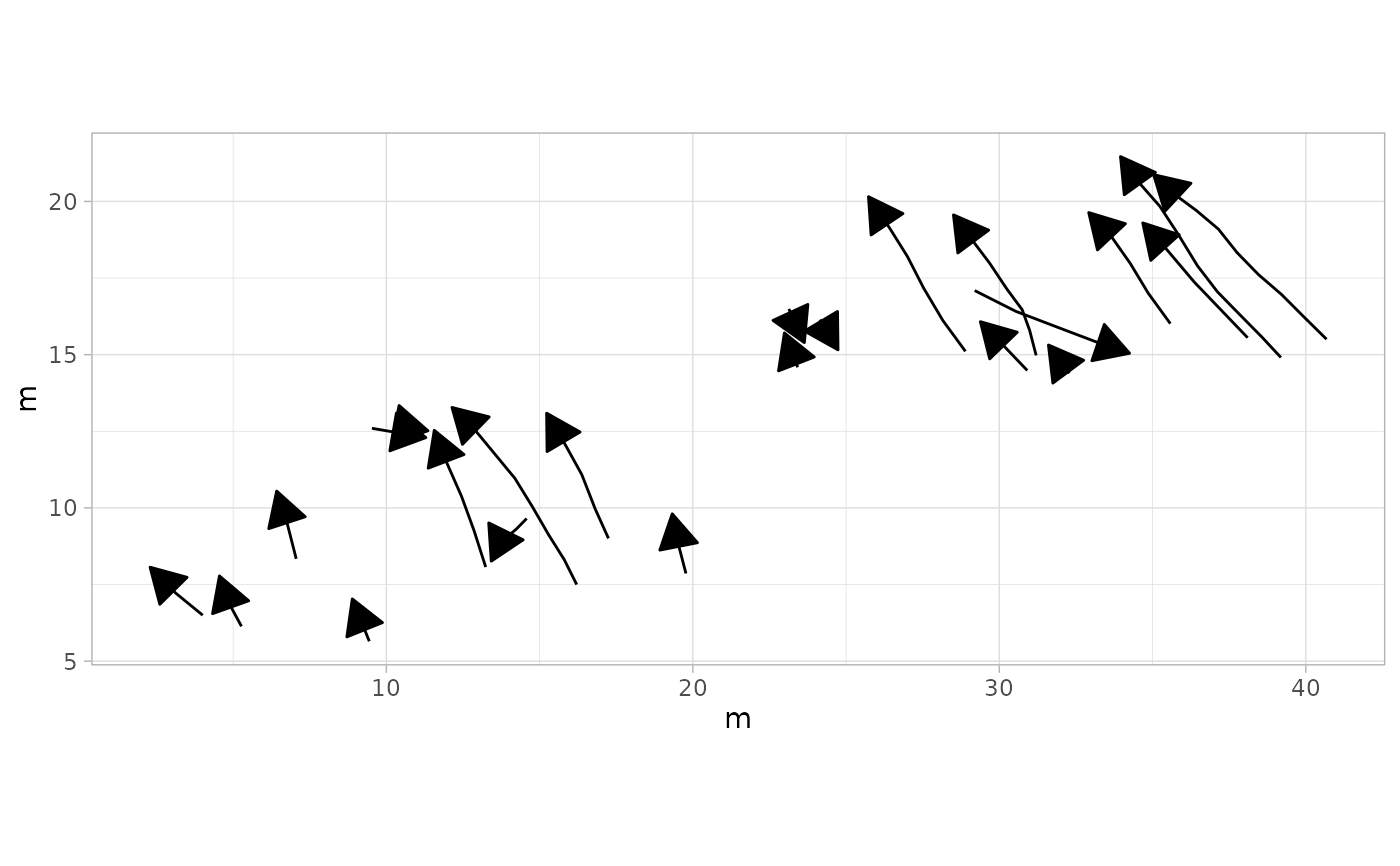
 # Example 13: Add arrowheads to show trajectory direction
plot_track(MountTom, plot = "Trajectories", arrow.t = TRUE, arrow.size = 0.2)
# Example 13: Add arrowheads to show trajectory direction
plot_track(MountTom, plot = "Trajectories", arrow.t = TRUE, arrow.size = 0.2)
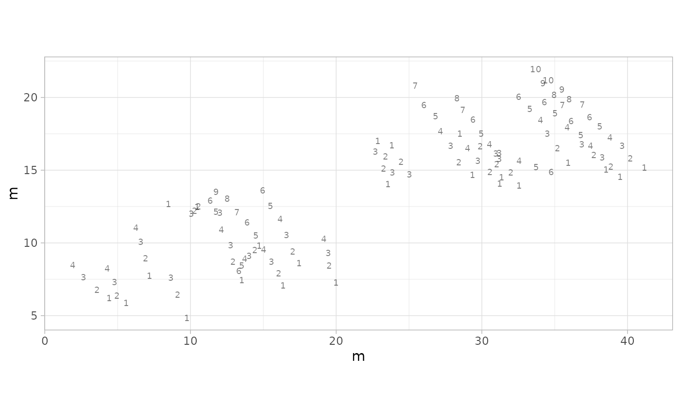
 # Example 14: Show footprint sequence numbers (quality control)
plot_track(MountTom, plot = "Footprints", seq.foot = TRUE)
# Example 14: Show footprint sequence numbers (quality control)
plot_track(MountTom, plot = "Footprints", seq.foot = TRUE)